At Simplexity, part of our work is designing embedded motion systems. As embedded motion engineers, we have to know how the smart electronics get placed within the physical structure (“embedded”) and how each component moves relative to each other (“motion”). In this three-part series, I delve into how we describe and model the latter term, motion, which we often take for granted as being quite simple.
In my introduction to 3D motion analysis, I discussed why it’s important to analyze motion, and I provided a simple 2D gear example. In that 2D example, each of the rotating components was rotating through a single angle, rotating about a single axis, and rotating about its center of mass. It was reasonable to say that ![]() and that
and that ![]() .
.
In this post, I explain why those simple relations aren’t universal, and why we have to be cautious when using them to help solve engineering problems.
Moving to 3D
What do we do when we encounter 3D motion systems that have parts rotating in more than one direction and not about their center of mass? How do we define what the angles are, and what is the angular velocity? Is it still something like ![]() ? Could we still use the relationship
? Could we still use the relationship ![]() ?
?
The motion of a quadcopter is a suitable example of a more complicated 3D motion system. It’s possible for a quadcopter in flight to translate in x, y, and z directions and rotate about x, y, and z (where x-y-z are three orthogonal directions fixed in the space). Ultimately, we want to finesse where the quadcopter goes and how it gets there (i.e., we want stable control over its position and orientation in the space).
To keep the quadcopter stable, we’ll use a gyroscope to measure the angular velocity about each axis, and feed that information back into the control algorithm. A 3-axis gyroscope will spit out three values for angular velocity, but note that these angular velocities correspond to axes that are fixed on the quadcopter. These x-y-z axes are not the same as the x-y-z axes that relate back to the quadcopter’s position, velocity, and acceleration in space. The conversion, so to speak, of the gyroscope’s angular velocity information into something digestible by the control algorithm is where the 3D dynamics model comes in handy.
Getting started with a more powerful 3D model
A more robust model of 3D motion starts with:
- Assigning a reference frame to a point fixed in your space.
- Treating all the objects in your system as rigid bodies.
- Assigning a reference frame to a certain point on each body.
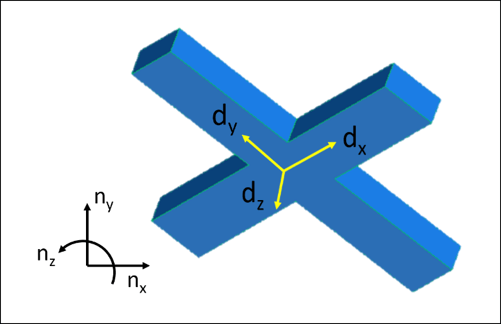
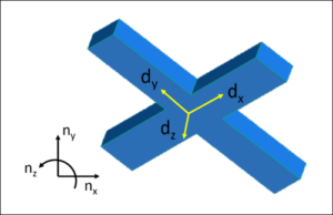
A reference frame is what I’m calling a set of three orthogonal unit vectors attached to a certain point. For our quadcopter example, the only object is the quadcopter, so we’ll treat that as a single rigid body. (We’ll ignore the other parts on the quadcopter here.) We’ll say that a reference frame N is fixed at a point on the earth and is made up of ![]() ,
, ![]() , and
, and ![]() . We’ll attach a reference frame D to the center of mass of the quadcopter. Reference frame D is made up of
. We’ll attach a reference frame D to the center of mass of the quadcopter. Reference frame D is made up of ![]() ,
, ![]() ,
, ![]() and . The diagram above shows a simplified quadcopter in CAD with D attached to its center of mass, and another reference frame N fixed in the space (
and . The diagram above shows a simplified quadcopter in CAD with D attached to its center of mass, and another reference frame N fixed in the space ( ![]() is pointing directly out of the page).
is pointing directly out of the page).
The measurements from the gyroscopes will give us angular velocities about ![]() ,
, ![]() ,
, ![]() and , and for the control algorithm, we’ll want to know how these values relate to meaningful angles in
and , and for the control algorithm, we’ll want to know how these values relate to meaningful angles in ![]() ,
, ![]() , and
, and ![]() . One way to achieve this is by defining the quadcopter’s orientation with a series of simple rotations about axes fixed on the quadcopter body. At the beginning of this step, we can express the angular velocity of the quadcopter in
. One way to achieve this is by defining the quadcopter’s orientation with a series of simple rotations about axes fixed on the quadcopter body. At the beginning of this step, we can express the angular velocity of the quadcopter in ![]() ,
, ![]() , and
, and ![]() , and it will look something like:
, and it will look something like: ![]() . At the end of this work, we’ll use rotation matrices to express each of the angular velocities in terms of Euler angles. Euler angles provide us one way of precisely describing the orientation of a body in 3D space. (Note that Euler angles don’t necessarily correspond to what we call yaw, pitch, and roll.) We will finish with precise expressions for
. At the end of this work, we’ll use rotation matrices to express each of the angular velocities in terms of Euler angles. Euler angles provide us one way of precisely describing the orientation of a body in 3D space. (Note that Euler angles don’t necessarily correspond to what we call yaw, pitch, and roll.) We will finish with precise expressions for ![]() ,
, ![]() , and
, and ![]() .
.
Since the quadcopter can rotate about more than one axis, we no longer have a simple ![]() ̇ relationship, and we can’t use
̇ relationship, and we can’t use ![]() to generally describe the velocity of a point on a quadcopter. In fact, an equation for
to generally describe the velocity of a point on a quadcopter. In fact, an equation for ![]() looks like:
looks like: ![]() , where
, where ![]() ,
, ![]() , and
, and ![]() are the Euler angles. The equations for
are the Euler angles. The equations for ![]() and
and ![]() are no less messy, unfortunately. For more details on these calculations, see the extra credit section.
are no less messy, unfortunately. For more details on these calculations, see the extra credit section.
In the final post in this series, I will discuss some important considerations when using a model like the one described in the above example. Please subscribe to Simplexity’s blog to get updates on future blog posts.
Extra credit
Here is one way to precisely define rotational information for the quadcopter:
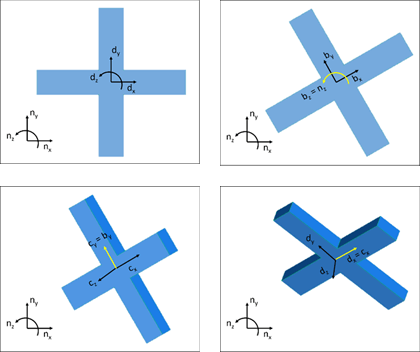
We’ll use intermediate reference frames to describe the orientation of the quadcopter. We’ll call the initial reference frame attached to the quadcopter B. Initially, ![]() ,
, ![]() , and
, and ![]() . Reference frame D is still attached to the body, and initially,
. Reference frame D is still attached to the body, and initially, ![]() . We will rotate first about
. We will rotate first about ![]() (which here is equal to
(which here is equal to ![]() ), and we will rotate by angle
), and we will rotate by angle ![]() . We can then write that B’s angular velocity in N is
. We can then write that B’s angular velocity in N is ![]() .
.
We will then rotate about another fixed axis on the body, ![]() , and we’ll call this new intermediate reference frame C. Initially,
, and we’ll call this new intermediate reference frame C. Initially,![]() ,
, ![]() , and
, and ![]() . We’ll rotate by angle
. We’ll rotate by angle ![]() about
about ![]() . We can then write that C’s angular velocity in B is
. We can then write that C’s angular velocity in B is ![]() .
.
Last, we will rotate about the fixed axis ![]() . Initially,
. Initially, ![]() ,
, ![]() , and
, and ![]() .We’ll rotate by angle
.We’ll rotate by angle ![]() about
about ![]() . We can then write that D’s angular velocity in C is
. We can then write that D’s angular velocity in C is ![]() .
.
From here, D’s angular velocity in N can be expressed as ![]() . However, this expression isn’t very useful yet in putting together dynamic equations. We already know that
. However, this expression isn’t very useful yet in putting together dynamic equations. We already know that ![]() because that’s the format of the data coming from the gyroscope. We’d like to re-express
because that’s the format of the data coming from the gyroscope. We’d like to re-express ![]() ,
, ![]() , and
, and ![]() in terms of our precise definition above.
in terms of our precise definition above.
Thankfully, each of those rotations created a rotation matrix between each of the intermediate frames, and we can use the multiplication of those rotation matrices to express ![]() in terms of our defined angles. (I won’t go into details with this part, but it comes straight out of making those intermediate rotations.) The result is the following:
in terms of our defined angles. (I won’t go into details with this part, but it comes straight out of making those intermediate rotations.) The result is the following:
![]()
From here, we see that ![]() is equal to the expression in front of
is equal to the expression in front of ![]() ,
, ![]() in front of
in front of ![]() , and
, and ![]() in front of
in front of ![]() .
.
Alas, our first step in giving a precise definition for the angular velocity of the quadcopter and making it usable by the control algorithm is complete.